Unveiling the Secrets of Cinema Revenue Success

Introduction

As a seasoned professional with over two decades of experience in accounting and robust expertise in data science, I bring a unique analytical perspective to financial analysis. This project on cinema sales data draws from my extensive background in financial management and revenue recognition, applying advanced analytics to uncover key drivers of cinema sales and optimize business strategies.

Enhancing the Project with Professional Experience

My extensive experience in accounting and revenue management significantly enhanced the execution of this project:

• Revenue Management Expertise: Managing revenue for SaaS and software companies required rigorous data analysis and forecasting skills, directly applicable to analyzing cinema revenue.
• Automation and Efficiency: Leading software implementations and automating accounting processes honed my ability to streamline workflows and handle large datasets, which was critical in this project.
• Analytical Skills: My background in performing variance analysis, revenue forecasts, and fair value assessments provided a strong foundation for developing and interpreting machine learning models.
• Technical Proficiency: Proficiency in SQL, Python, and R, gained through years of professional experience and data science education, enabled me to efficiently clean, preprocess, and model the cinema data.

Technologies and Tools Used

Enhanced by my recent certification as a Certified Data Science Professional in Python from DataCamp, my advanced Python skills were pivotal in this project. Utilizing libraries like NumPy, pandas, matplotlib, scikit-learn, and Seaborn, I conducted sophisticated data manipulations, statistical modeling, and insightful visualizations.

Project Objectives

This project aims to leverage deep insights from accounting and data science to understand and amplify the factors influencing cinema sales, thereby boosting revenue potential.

Dataset Overview

The dataset for this project was sourced from Kaggle at Cinema Ticket Offers. It encompasses detailed records of ticket sales, seating capacities, show timings, and other pertinent data, amounting to over 142,000 transaction records across various cinema and film codes. This rich dataset provides the foundation for a comprehensive analysis aimed at uncovering underlying sales drivers.

Key Features Include:

• film_code: Unique identifier for each film shown.
• cinema_code: Unique identifier for each cinema venue.
• total_sales: Total revenue generated from each screening.
• tickets_sold: Number of tickets sold for each show.
• tickets_out: Count of tickets that were canceled.
• show_time: Schedule for each film screening.
• occu_perc: Percentage of occupied seats in the cinema.
• ticket_price: Cost of tickets for each show.
• ticket_use: Actual number of tickets used by the audience.
• capacity: Seating capacity of the cinema.
• date: Specific date of each screening.
• month: Month in which the screening took place.
• quarter: Business quarter of each screening event.
• day: Day of the week the film was shown.

Methodology

Exploratory Data Analysis (EDA)

Through extensive exploratory analysis, I identified crucial patterns and variables, ensuring the accuracy of data type conversions and analyses, which are fundamental to the success of this project.

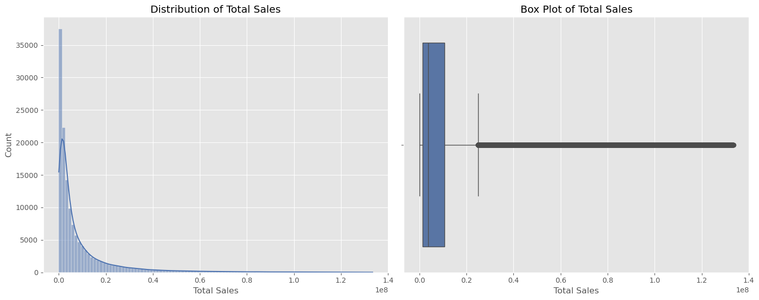Figure 1: Histogram and boxplot showing the distribution of total sales.

The histogram shows a right-skewed distribution. Most cinema showings have relatively low total sales, with a few showings achieving very high sales. The box plot reveals numerous outliers on the higher end of total sales. These outliers represent cinema showings with exceptionally high sales compared to the typical range. The skewness in the distribution suggests that while most of the cinema showings generate modest revenue, there are a significant number of showings (possibly big-ticket films or special screenings) that generate much higher sales. The presence of outliers indicates that certain events or movies might be extremely popular, driving exceptionally high sales.

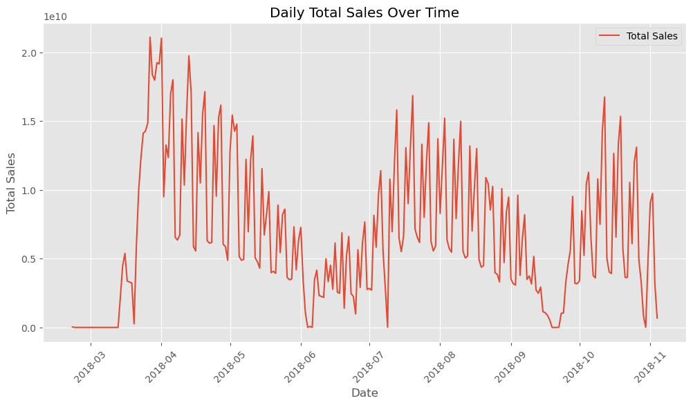Figure 2: The line graph traces daily total sales, offering insight into the sales trends over time and helping to identify periods of high and low demand.

The plot shows the number of records in the dataset resampled by day. It illustrates the daily distribution of the data, providing a visual indication of any fluctuations or trends in the number of records over time.

Data Preprocessing

Significant adjustments made to ensure data quality included:

• Filling Missing Values: Addressing gaps in the ‘capacity’ data by applying average values. My background in financial forecasting and analysis was crucial in determining the most statistically appropriate method for handling missing data.

• Adjusting Show Times: Standardizing show times to a 24-hour format, leveraging my expertise in ensuring data accuracy and compliance with financial standards.

# Adjust showtime for validity
# Subtract 12 from show_time values between 13 and 24
df.loc[(df['show_time'] > 12) & (df['show_time'] <= 24), 'show_time'] -= 12

# Drop rows where 'show_time' exceeds 24
df = df[df['show_time'] <= 24]

• Handling Overcapacity: Correcting any instances where occupancy percentages exceeded plausible limits, a task aligned with financial auditing practices where accuracy and regulatory compliance are paramount.

# Fill negative theater capacity values with mean for that cinema_code

# Calculate the mean capacity for each cinema_code, excluding negative values
mean_capacity_per_cinema = df[df['capacity'] > 0].groupby('cinema_code')['capacity'].mean()

# Fill negative capacity values with the mean capacity of the corresponding cinema_code
df.loc[df['capacity'] < 0, 'capacity'] = df.loc[df['capacity'] < 0, 'cinema_code'].apply(
    lambda x: mean_capacity_per_cinema.get(x, np.nan)
)

# Handle cases where mean capacity is not available
df['capacity'].fillna(df['capacity'].mean(), inplace=True)

# Check if there are any negative values remaining in capacity
remaining_negative_capacity = df[df['capacity'] < 0].shape[0]

print(remaining_negative_capacity)

• Encoding Categorical Variables: Converting categorical data into numeric formats, a skill honed through my experience with financial databases and ensuring compliance with data standards.

# Use category encoders to encode categorical variables; otherwise too many features to handle (over 300)
import category_encoders as ce

# List of categorical columns to be binary encoded
categorical_columns = ['film_code', 'cinema_code', 'month', 'day']

# Create a Binary Encoder
binary_encoder = ce.BinaryEncoder(cols=categorical_columns)

# Fit and transform to produce binary encoded DataFrame
df_encoded = binary_encoder.fit_transform(df)

# Display the first few rows of the encoded DataFrame
df_encoded.head()

• Eliminating Highly Correlated Features: Identifying and removing features with high correlation to prevent multicollinearity, ensuring the model’s robustness and interpretability.

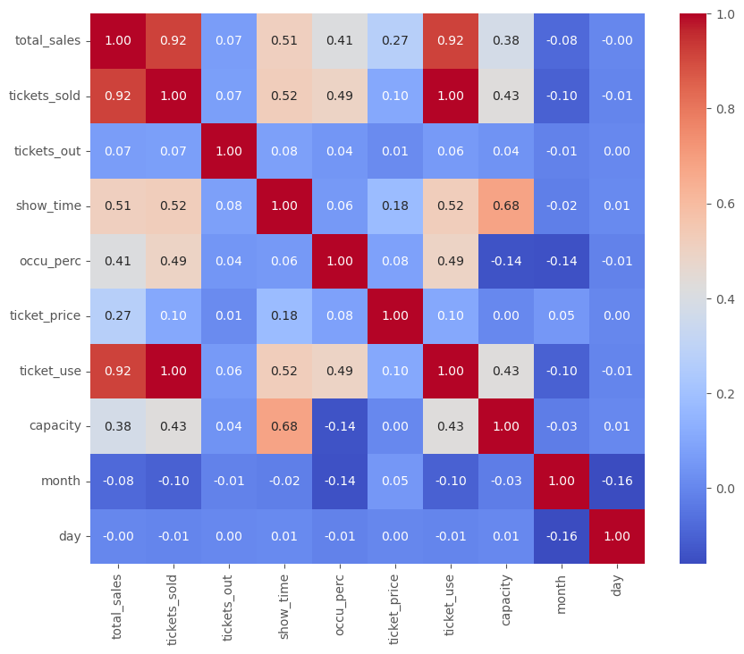Figure 3: The correlation heatmap highlights the multicollinearity among features.

Modeling

Various machine learning models were employed to predict cinema revenue, including Random Forest and Gradient Boosting. Model selection was based on performance metrics such as R-squared and Mean Absolute Error (MAE). Hyperparameter tuning was conducted to optimize model performance.

# Define parameter grid for random forest
param_grid = {
    'n_estimators': [100, 300, 500], 
    'max_features': ['sqrt', 'log2'],  
    'max_depth': [5, 10, 20, 50],  
    'min_samples_split': [2, 3, 5, 10],  
    'min_samples_leaf': [1, 2, 3, 4],  
    'bootstrap': [True, False]  # Limited to one option for simplicity
}

# Create base model to tune
rf = RandomForestRegressor()

# Set Randomized Search parameters
rf_random = RandomizedSearchCV(estimator=rf, param_distributions=param_grid, n_iter=20, cv=3, verbose=2, random_state=42, n_jobs=-1)  # later increase iterations

# Fit the random search model
rf_random.fit(X_train, y_train)

# Print the best parameters
best_params = rf_random.best_params_
print(f"Best Parameters: {best_params}")

Model Results

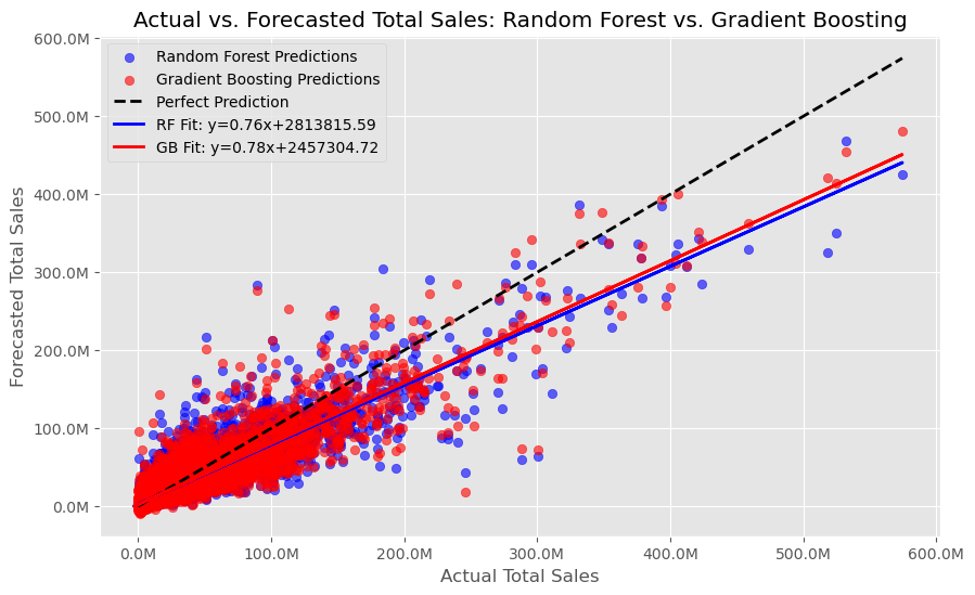Figure 4: Scatter plot comparing predicted sales against actual sales, demonstrating the accuracy of the Random Forest model.

The figure visually demonstrates that both Random Forest and Gradient Boosting models provide reasonable predictions of total sales, with similar trends and levels of accuracy. The regression lines and the scatter plots help in understanding the models’ predictive behavior and areas where they may need further tuning or improvement.

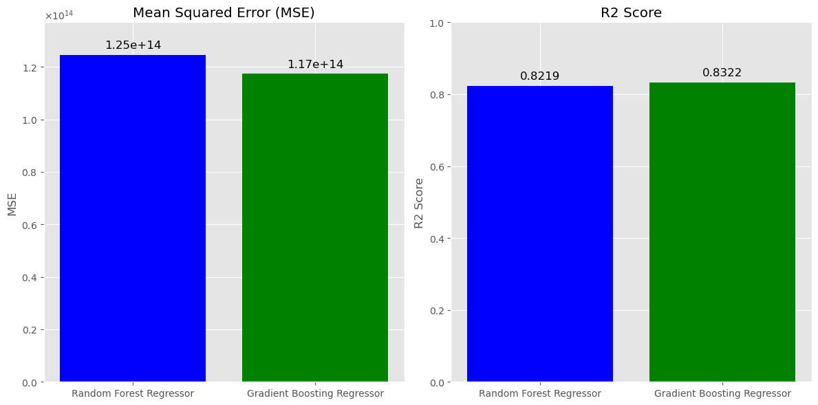Figure 5: Bar plot displaying MSE and R-squared for the RF and GB models.

The MSE for the Random Forest model is marginally higher than for the Gradient Boosting model. Since MSE measures the average squared difference between the predicted and actual values, a lower MSE is better. This suggests that the Gradient Boosting model has a slight edge in terms of predictive accuracy. Both models have very similar R2 scores, with the Gradient Boosting model having a slight advantage.

The models provided valuable insights into the factors influencing cinema revenue. Key features such as ticket price, occupancy rate, and show timing were identified as significant predictors of revenue.

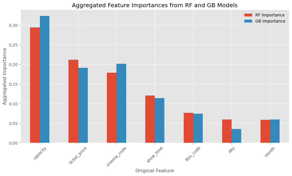Figure 6: Bar chart displaying aggregated feature importances from RF and GB models, highlighting the predictive power of features such as capacity, ticket price, and cinema code.

From these results, we can infer that the physical constraints and pricing (capacity and ticket price) are the most influential predictors. However, the specific cinema and showtime also play a role, potentially due to different cinema sizes, locations, or time-specific demand. Furthermore, while the film itself and the day of the showing have some predictive power, they are less critical than the aforementioned features. Lastly, the month seems to have the least predictive power, which might suggest that the target variable is not strongly seasonal, or other features already capture the variance that month would otherwise explain.

Key Insights and Actionable Strategies

• Pricing Optimization: Recommended dynamic pricing models to maximize earnings based on time and film type.
• Capacity Utilization: Provided strategic scheduling recommendations to enhance seat utilization.
• Targeted Marketing: Developed marketing strategies focused on the most influential factors affecting customer attendance and preferences.
• Show-Time Optimization: Proposed adjustments to show times based on patterns that maximize attendance and revenue.

Challenges and Learning Experience

This project was a valuable learning experience, highlighting the intersection of data science and business strategy. Some of the key challenges and learnings include:

• Integration of Domain Knowledge: Applying my extensive background in revenue management to frame the data science problem provided a unique perspective and enhanced the model’s relevance.
• Advanced Analytics: Utilizing machine learning models such as Random Forest and Gradient Boosting deepened my understanding of their capabilities and limitations.
• Communication of Insights: Translating complex model outputs into actionable business recommendations reinforced the importance of clear and concise communication in data science.

Conclusion

This analysis provides a detailed look at the factors driving cinema sales, utilizing a comprehensive dataset and advanced machine learning methods. The insights gained can help optimize ticket pricing, scheduling, and overall cinema management strategies. My transition from a CPA to a data scientist allows me to combine financial acumen with technical expertise, offering a unique perspective on data-driven decision-making.

Discover the Full Story

For those interested in the technical details, including the complete code and methodologies, view the project notebook on NBViewer.