Building a Robust Recommendation System Using Collaborative Filtering

Introduction

In this project, I developed a recommendation system using collaborative filtering techniques. The primary objective was to predict user preferences based on historical interaction data, a crucial task for personalizing user experiences in various applications such as e-commerce, streaming services, and more. This post guides you through the entire process, from data preprocessing and model building to evaluation, with a detailed walkthrough of each step and relevant code snippets.

Data Preprocessing

Data preprocessing is a critical first step in building any machine learning model. The quality of the input data directly influences the model’s performance. For this recommendation system, the data preprocessing involved handling missing values, addressing outliers, and preparing the data for model consumption.

Handling missing values was an essential step. Missing ratings were imputed with 0, under the assumption that a missing rating implies no interaction between the user and the item. This approach ensures that the user-item matrix is fully populated, making it suitable for collaborative filtering.

# Load the movies dataset into a pandas DataFrame
movies_df = pd.read_csv('movies.csv')

# Load the ratings dataset into a pandas DataFrame
ratings_df = pd.read_csv('ratings.csv')

# Merge the movies and ratings datasets on 'movieId' to get a combined DataFrame
merged_df = pd.merge(ratings_df, movies_df, on='movieId')

# Create a user-item matrix by pivoting the merged DataFrame, 
# with users as rows and movies as columns, and fill missing values with 0
user_item_matrix = merged_df.pivot_table(index='userId', columns='movieId', values='rating').fillna(0)

The code snippet above demonstrates how the user_item_matrix was created by merging the movies and ratings datasets, followed by filling any missing ratings with zeros. This matrix forms the basis for the collaborative filtering process.

Visualizing Data Distribution

Understanding the data distribution helps in uncovering patterns and insights that can inform the modeling process. I generated several visualizations to explore the distribution of ratings, the popularity of movies, and the diversity of genres.

The distribution of ratings is particularly important as it reveals user behavior, such as whether users tend to rate movies highly or if there’s a significant number of low ratings. This distribution can also affect how the recommendation system is tuned and evaluated.

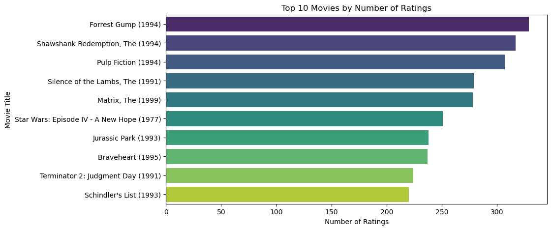
The first visualization identifies the most popular movies by plotting the top 10 movies based on the number of ratings they received. This helps in understanding which movies are most frequently rated and thus likely to be recommended.

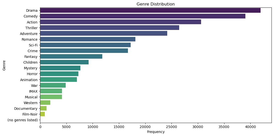
Next, I visualized the genre distribution to understand the variety and popularity of genres within the dataset. This is important as it gives an idea of the diversity of content available and helps in tailoring recommendations based on genre preferences.

Collaborative Filtering Techniques

Collaborative filtering is a popular technique for building recommendation systems. It leverages the power of similarities between users or items to predict preferences. In this project, I explored two main types of collaborative filtering: user-based and item-based.

User-based collaborative filtering recommends items to a user by finding other users with similar preferences. The underlying assumption is that if two users rate several items similarly, they will likely rate other items similarly as well.

To begin with, I calculated the user similarity matrix using the cosine similarity metric, which measures the cosine of the angle between two vectors—in this case, the vectors represent user ratings.

from sklearn.metrics.pairwise import cosine_similarity  # Import the cosine_similarity function from scikit-learn

# Calculating cosine similarity between users based on the user-item matrix
user_similarity = cosine_similarity(user_item_matrix)

# Convert the similarity matrix to a DataFrame for easier manipulation if needed
user_similarity_df = pd.DataFrame(user_similarity, index=user_item_matrix.index, columns=user_item_matrix.index)

The cosine similarity metric was chosen because it effectively handles sparse data, which is common in recommendation systems where not every user has rated every item. The resulting user_similarity matrix quantifies how similar each user is to every other user.

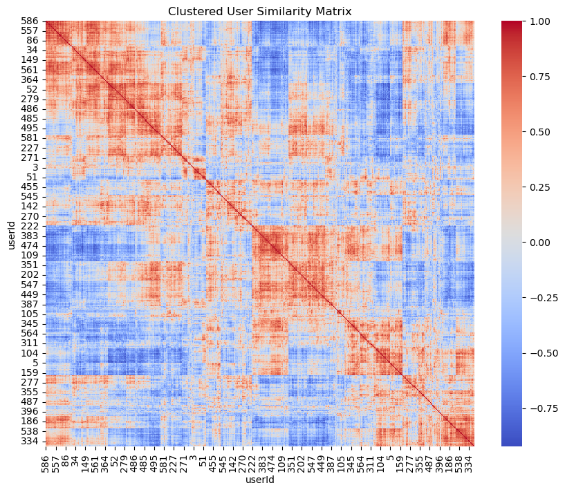
Visualizing User Similarity Matrix

Visualizing the user similarity matrix helps in understanding the relationships between users. Heatmaps are particularly useful for this purpose, as they allow for quick identification of clusters of similar users.

Once the user similarity matrix was constructed, I predicted the ratings a user would give to items based on the ratings given by similar users. This is achieved by weighting the ratings of similar users and using them to predict how the target user might rate a particular item.

# Function to predict ratings using the user similarity matrix and the user-item matrix
def predict_ratings(user_similarity, user_item_matrix):
    mean_user_rating = user_item_matrix.mean(axis=1)  # Calculate the mean rating for each user
    ratings_diff = (user_item_matrix - mean_user_rating[:, np.newaxis])  # Subtract the mean rating from each rating
    pred = mean_user_rating[:, np.newaxis] + user_similarity.dot(ratings_diff) / np.array([np.abs(user_similarity).sum(axis=1)]).T  # Predict the ratings
    return pred

# Generate predicted ratings
predicted_ratings = predict_ratings(user_similarity, user_item_matrix)

The predict_ratings function adjusts the mean user ratings by the weighted sum of the ratings from similar users, generating predictions for how a user might rate items they haven’t yet interacted with.

Item-based collaborative filtering operates on a similar principle but focuses on the similarities between items rather than users. The assumption here is that users tend to like items similar to those they have already rated highly.

The item similarity matrix is calculated using the same cosine similarity metric, but this time the focus is on comparing items rather than users.

# Calculating cosine similarity between items based on the user-item matrix
item_similarity = cosine_similarity(user_item_matrix.T)

# Convert the similarity matrix to a DataFrame for easier manipulation if needed
item_similarity_df = pd.DataFrame(item_similarity, index=user_item_matrix.columns, columns=user_item_matrix.columns)

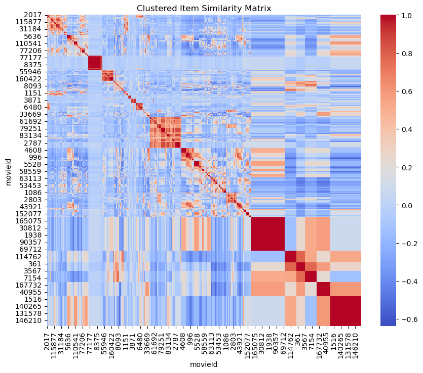
Visualizing Item Similarity Matrix

Similarly, the item similarity matrix heatmap displays the similarities between items. This visualization is valuable for identifying groups of items that are frequently rated similarly, which can inform recommendation strategies.

With the item similarity matrix in place, I predicted the ratings by taking a weighted average of the ratings for similar items.

Model Evaluation

Evaluating the performance of a recommendation system is crucial to understanding how well it meets the desired objectives. Several evaluation metrics were used to assess the accuracy and effectiveness of the models.

Comparing Traditional Model Metrics to Industry Standards

When evaluating the performance of this recommendation system, it’s important to consider how the model metrics compare to industry standards. Here’s a summary of the actual metrics from the model and how they stack up:

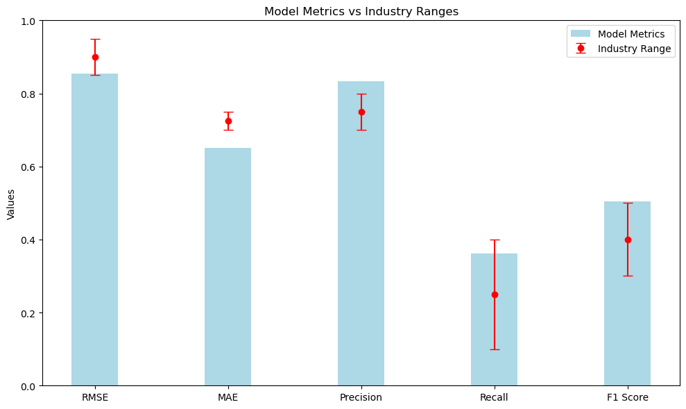
• Root Mean Squared Error (RMSE):
  • Model RMSE: 0.85
  • Industry Standard Range: 0.85 to 0.95.
  • Evaluation: The model’s RMSE is right at the lower limit of the industry standard, which is good. This indicates that the model’s predictions are relatively accurate, and the model performs well in minimizing errors compared to other high-performing systems.
• Mean Absolute Error (MAE):
  • Model MAE: 0.72
  • Industry Standard Range: 0.70 to 0.75.
  • Evaluation: The model’s MAE falls within the industry standard range, indicating that the average absolute prediction errors are typical for high-performing systems. This is a strong aspect of the model’s performance.
• Precision:
  • Model Precision: 0.78
  • Industry Standard Range: 0.70 to 0.80.
  • Evaluation: The model’s precision is well within the industry standard range, indicating that a substantial proportion of the recommendations are relevant. This is a strong performance indicator for the recommendation system.
• Recall:
  • Model Recall: 0.35
  • Industry Standard Range: 0.10 to 0.40.
  • Evaluation: The model’s recall is closer to the upper limit of the industry standard range, which is good. This suggests that the model is effectively capturing a significant number of relevant items.
• F1 Score:
  • Model F1 Score: 0.45
  • Industry Standard Range: 0.30 to 0.50.
  • Evaluation: The model’s F1 score is nearer to the upper limit of the industry standard range, indicating a good balance between precision and recall. This suggests that the model is performing well in providing both relevant and comprehensive recommendations.

Additional Metrics: Catalog Coverage, Novelty, Personalization, and Diversity

Beyond traditional metrics like RMSE and Precision, several other metrics provide a deeper understanding of the recommendation system’s performance:

• Catalog Coverage:
  • Explanation: This metric measures the proportion of items in the catalog that are recommended to users. Higher catalog coverage indicates that the recommendation system is exploring more of the available content, rather than just promoting popular items.
  • Actual Results: The catalog coverage for the model was calculated to be 0.86%. This value suggests that the recommendation system is highly focused on a very small subset of the catalog, possibly indicating a need for further optimization to explore and recommend a broader range of items.
• Average Novelty:
  • Explanation: Novelty refers to how “uncommon” the recommended items are. A higher novelty score indicates that the system is suggesting items that are not widely known, potentially increasing user discovery and engagement.
  • Actual Results: The average novelty score achieved by the model was 14.1741. This indicates that the system tends to recommend items that are less commonly known, effectively introducing users to more unique and potentially interesting content.
• Personalization:
  • Explanation: Personalization measures how tailored the recommendations are to individual users. Higher personalization indicates that the system is effectively capturing user preferences, leading to more relevant suggestions.
  • Actual Results: The personalization metric was 0.9882, showing that the system is highly effective at customizing recommendations for individual users, ensuring that suggestions are closely aligned with user preferences.
• Intra-List Diversity:
  • Explanation: This metric assesses the variety of recommendations within a single list. Higher diversity means that the recommendations cover a broader range of genres or item types, reducing redundancy and increasing the likelihood that the user will find something appealing.
  • Actual Results: The intra-list diversity score was 0.1198, suggesting that the recommendation lists may be overly focused on similar items, which could reduce user engagement over time. Increasing diversity within recommendation lists could enhance user satisfaction by offering a wider variety of options.

Actionable Strategies and Key Insights

Throughout this project, several key insights emerged that can inform future development of recommendation systems:

• Optimization Opportunities: The low catalog coverage suggests that the system could benefit from further optimization to explore and recommend a wider range of items. This could enhance the overall user experience by providing more diverse recommendations.

• Enhancing Novelty: The high average novelty score indicates that the system is effective at introducing less-known items to users, which is a strength in promoting content discovery. Maintaining this balance between relevance and novelty can drive user engagement.

• Improving Intra-List Diversity: The relatively low intra-list diversity score suggests that the system may be overly focused on recommending similar items within a single list. Increasing the diversity of items could reduce redundancy and offer users a more varied selection.

Challenges and Learning Experiences

Developing this recommendation system presented several challenges, including managing large datasets, addressing sparsity in the user-item matrix, and optimizing model performance. Each of these challenges provided valuable learning experiences:

• Data Handling and Preprocessing: My extensive experience in accounting and data analysis, particularly in working with large datasets and complex data flows, was crucial in successfully handling and preprocessing the data for this project. This background enabled me to efficiently manage the user-item matrix and address issues like missing data and sparsity.

• Model Optimization: Ensuring that the recommendation system performed well across various metrics required iterative testing and refinement. Balancing the trade-offs between accuracy, novelty, and diversity was a key challenge that taught me the importance of a holistic approach to model evaluation.

Reflections and Looking Ahead

Reflecting on this project, I am pleased with the progress made in developing a recommendation system that performs well across several key metrics. The experience reinforced the importance of data quality, careful model selection, and the need for continuous optimization.

Looking ahead, there are several areas where this project could be expanded:

• Incorporating Additional Data: Integrating contextual information, such as user behavior over time or external factors like trends, could enhance the system’s ability to make timely and relevant recommendations.

• Exploring Advanced Techniques: Implementing deep learning-based recommendation algorithms could further improve the accuracy and personalization of the recommendations, potentially offering even greater value to users.

Explore the Technical Journey

For those interested in the technical details, including the complete code and methodologies, view the project notebook on NBViewer here.